Carlos, director of a gardening company with 15 employees, knew that his sales fluctuated according to the seasons, but he had never quantified exactly when and how much. Every spring he ran out of stock of key products, while every winter he accumulated inventory that didn't move until months later. His accountant suggested hiring more staff in summer, but he wasn't sure exactly when or for how long.
Carlos's story is that of thousands of SMEs that operate 'blindly' regarding the temporal patterns of their business. Time series analysis converts those hidden patterns into actionable information, enabling strategic planning based on real data instead of intuition.
What is Time Series Analysis?
A time series is simply a sequence of chronologically ordered data: monthly sales, daily number of customers, quarterly revenue, weekly website visits. Time series analysis studies this data to identify patterns, trends, and cycles that allow predicting future values.
For an SME, this means transforming historical data it already possesses into strategic information for making planning, hiring, purchasing, marketing, and operations decisions. It's like having a time machine that reveals what to expect in the coming months based on what has already happened.
The Four Fundamental Components
Every business time series can be decomposed into four basic elements that, once identified, allow complete understanding of business behavior and making accurate predictions.
1. Trend: The General Direction
The trend shows whether your business is growing, stagnant, or declining in the long term. It's the underlying pattern when we remove daily, weekly, or seasonal fluctuations.
- Growing trend: Sales increase consistently month after month
- Declining trend: Gradual decline in product demand
- Stable trend: Mature business with horizontal growth
- Cyclical trend: Growth and decline in long periods (2-10 years)
2. Seasonality: Predictable Patterns
Demand seasonality are regular and predictable fluctuations that repeat in specific periods: daily, weekly, monthly, or annual.
| Business Type | Seasonal Pattern | Practical Example |
|---|---|---|
| Fashion retail | Annual | Peaks in spring/autumn, decline in January |
| Restaurant | Weekly | Maximum Friday-Sunday, minimum Monday-Tuesday |
| E-commerce | Daily | Peaks 8:00-10:00 PM, minimum 4:00-6:00 AM |
| Tourism | Annual | Maximum summer, minimum winter |
| B2B services | Monthly | Decline in August and December |
| Financial products | Quarterly | Peaks at the end of each quarter |
3. Cycles: Irregular Fluctuations
Cycles are fluctuations that don't have a fixed periodicity like seasonality. They are influenced by economic factors, industry changes, or external events.
- Economic cycles: Recessions, expansions, financial crises
- Technological cycles: Adoption of new technologies, obsolescence
- Competitive cycles: Entry of new competitors, price wars
- Regulatory cycles: Changes in laws, regulations, taxes
4. Noise: Random Variations
Noise are random fluctuations that don't follow any identifiable pattern. They represent unique events, measurement errors, or unpredictable factors.
The goal of time series analysis is to separate these components to understand what is predictable (trend, seasonality) and what is random (noise), allowing for more accurate projections.
Practical Use Cases for SMEs
Business trend analysis has immediate applications in multiple areas of any SME. Each department can benefit from more accurate predictions to optimize resources and planning.
Sales and Marketing Planning
- Monthly/quarterly revenue prediction for budgets
- Identification of high demand periods to intensify marketing
- Promotional campaign planning based on historical seasonality
- Advertising budget allocation according to conversion patterns
- Early detection of declines in specific products
Human Resources Management
- Temporary staff hiring for seasonal peaks
- Team vacation planning during low demand periods
- Work schedule adjustment according to activity patterns
- Variable payroll budget based on sales projections
- Identification of training needs according to business cycles
Financial Optimization
- Monthly cash flow prediction for liquidity management
- Investment planning during periods of higher profitability
- Credit line negotiation based on seasonal patterns
- Supplier payment optimization according to income cycles
- Financial reserves calculated according to historical variability
import pandas as pd
import numpy as np
import matplotlib.pyplot as plt
from statsmodels.tsa.seasonal import seasonal_decompose
from statsmodels.tsa.holtwinters import ExponentialSmoothing
from datetime import datetime, timedelta

class TimeSeriesAnalyzer:
    def __init__(self, data):
        """
        Initializes the analyzer with time series data
        data: DataFrame with 'date' and 'value' columns
        """
        self.data = data.copy()
        self.data['date'] = pd.to_datetime(self.data['date'])
        self.data = self.data.set_index('date').sort_index()
        self.components = None
        self.model = None

    def decompose_series(self, seasonal_period=12):
        """
        Decomposes the series into trend, seasonality, and noise
        """
        self.components = seasonal_decompose(
            self.data['value'],
            model='multiplicative',
            period=seasonal_period
        )

        return self.components

    def visualize_components(self):
        """
        Creates graphs of the series components
        """
        if self.components is None:
            self.decompose_series()

        fig, axes = plt.subplots(4, 1, figsize=(15, 12))

        # Original series
        self.components.observed.plot(ax=axes[0], title='Original Series')
        axes[0].set_ylabel('Value')

        # Trend
        self.components.trend.plot(ax=axes[1], title='Trend', color='orange')
        axes[1].set_ylabel('Trend')

        # Seasonality
        self.components.seasonal.plot(ax=axes[2], title='Seasonality', color='green')
        axes[2].set_ylabel('Seasonal Factor')

        # Noise
        self.components.resid.plot(ax=axes[3], title='Noise/Residuals', color='red')
        axes[3].set_ylabel('Residuals')

        plt.tight_layout()
        return fig

    def calculate_seasonal_statistics(self):
        """
        Calculates useful statistics about seasonality
        """
        if self.components is None:
            self.decompose_series()

        # Extract seasonal component
        seasonal = self.components.seasonal.dropna()

        # Calculate statistics by period
        statistics = {
            'maximum_factor': seasonal.max(),
            'minimum_factor': seasonal.min(),
            'seasonal_variation': seasonal.max() - seasonal.min(),
            'peak_period': seasonal.idxmax().month if hasattr(seasonal.idxmax(), 'month') else seasonal.idxmax(),
            'valley_period': seasonal.idxmin().month if hasattr(seasonal.idxmin(), 'month') else seasonal.idxmin(),
            'coefficient_variation': seasonal.std() / seasonal.mean()
        }

        return statistics

    def train_prediction_model(self, prediction_horizon=12):
        """
        Trains Holt-Winters model for prediction
        """
        # Determine if there's significant seasonality
        if self.components is None:
            self.decompose_series()

        statistics = self.calculate_seasonal_statistics()
        has_seasonality = statistics['coefficient_variation'] > 0.1

        # Configure model
        if has_seasonality:
            self.model = ExponentialSmoothing(
                self.data['value'],
                trend='add',
                seasonal='mul',
                seasonal_periods=12
            ).fit()
        else:
            self.model = ExponentialSmoothing(
                self.data['value'],
                trend='add'
            ).fit()

        # Make predictions
        predictions = self.model.forecast(prediction_horizon)

        # Calculate confidence intervals (approximate)
        error_std = np.std(self.model.resid)
        lower_interval = predictions - 1.96 * error_std
        upper_interval = predictions + 1.96 * error_std

        return {
            'predictions': predictions,
            'lower_interval': lower_interval,
            'upper_interval': upper_interval,
            'model_info': {
                'aic': self.model.aic,
                'has_seasonality': has_seasonality,
                'average_error': error_std
            }
        }

    def generate_insights_report(self):
        """
        Generates report with business insights
        """
        if self.components is None:
            self.decompose_series()

        statistics = self.calculate_seasonal_statistics()

        # Analyze trend
        trend = self.components.trend.dropna()
        annual_growth = ((trend.iloc[-12:].mean() / trend.iloc[:12].mean()) - 1) * 100

        # Volatility
        volatility = self.data['value'].pct_change().std() * 100

        report = {
            'trend_summary': {
                'annual_growth_pct': annual_growth,
                'direction': 'Growing' if annual_growth > 5 else 'Declining' if annual_growth < -5 else 'Stable'
            },
            'seasonality_summary': {
                'maximum_variation_pct': (statistics['seasonal_variation'] - 1) * 100,
                'peak_month': statistics['peak_period'],
                'valley_month': statistics['valley_period'],
                'is_significant': statistics['coefficient_variation'] > 0.1
            },
            'volatility': {
                'monthly_volatility_pct': volatility,
                'level': 'High' if volatility > 20 else 'Medium' if volatility > 10 else 'Low'
            },
            'recommendations': self._generate_recommendations(annual_growth, statistics, volatility)
        }

        return report

    def _generate_recommendations(self, growth, statistics, volatility):
        """
        Generates specific recommendations based on analysis
        """
        recommendations = []

        # Trend-based recommendations
        if growth > 10:
            recommendations.append("Consider expanding operational capacity to sustain growth")
            recommendations.append("Plan hiring additional staff")
        elif growth < -10:
            recommendations.append("Review commercial strategy - significant decline detected")
            recommendations.append("Consider product or market diversification")

        # Seasonality-based recommendations
        if statistics['coefficient_variation'] > 0.2:
            recommendations.append("Plan inventory and staff according to seasonal patterns")
            recommendations.append("Consider complementary products to stabilize income")

        # Volatility-based recommendations
        if volatility > 25:
            recommendations.append("Maintain financial reserves to manage high volatility")
            recommendations.append("Implement alert system for sudden changes")

        return recommendations

# Example usage with simulated data
np.random.seed(42)
dates = pd.date_range('2022-01-01', '2024-12-31', freq='M')

# Simulate series with trend, seasonality, and noise
trend = np.linspace(1000, 1500, len(dates))
seasonality = 100 * np.sin(2 * np.pi * np.arange(len(dates)) / 12)
noise = np.random.normal(0, 50, len(dates))
values = trend + seasonality + noise

example_data = pd.DataFrame({
    'date': dates,
    'value': values
})

# Create analyzer
analyzer = TimeSeriesAnalyzer(example_data)

# Decompose and analyze
components = analyzer.decompose_series()
report = analyzer.generate_insights_report()
predictions = analyzer.train_prediction_model(6)

print("=== TIME SERIES ANALYSIS REPORT ===")
print(f"Annual growth: {report['trend_summary']['annual_growth_pct']:.1f}%")
print(f"Direction: {report['trend_summary']['direction']}")
print(f"Maximum seasonal variation: {report['seasonality_summary']['maximum_variation_pct']:.1f}%")
print(f"Volatility: {report['volatility']['level']} ({report['volatility']['monthly_volatility_pct']:.1f}%)")
print("\nRecommendations:")
for rec in report['recommendations']:
    print(f"- {rec}")
Data Needed to Get Started
One of the advantages of time series analysis is that it uses data that most SMEs already collect routinely. You don't need to invest in new capture systems: your existing records contain valuable information waiting to be analyzed.
Essential Basic Data
| Data Type | Common Source | Minimum Frequency | Minimum Period |
|---|---|---|---|
| Sales/Revenue | Billing, POS, E-commerce | Daily | 12 months |
| Number of customers | CRM, Database | Weekly | 18 months |
| Inventory/Stock | ERP, Spreadsheets | Weekly | 12 months |
| Web visits/traffic | Google Analytics | Daily | 6 months |
| Operating costs | Accounting | Monthly | 24 months |
| Active staff | HR, Payroll | Monthly | 18 months |
Enriching Contextual Data
To improve prediction accuracy and better understand the factors that influence your business, it's recommended to include external variables:
- Commercial calendar: Holidays, long weekends, Black Friday, sales
- Weather data: Temperature, precipitation, seasonal indices
- Competitive activity: Launches, promotions, price changes
- Economic indicators: CPI, unemployment, consumer confidence
- Marketing events: Campaigns, advertising investment, media appearances
- Internal factors: Price changes, new products, expansions
Data Preparation and Cleaning
import pandas as pd
import numpy as np
from datetime import datetime

def prepare_time_series_data(data_file, date_column, value_column):
    """
    Prepares and cleans data for time series analysis
    """
    # Load data
    df = pd.read_csv(data_file)

    # Convert date
    df[date_column] = pd.to_datetime(df[date_column])

    # Sort by date
    df = df.sort_values(date_column)

    # Detect and handle missing values
    print(f"Missing values detected: {df[value_column].isnull().sum()}")

    # Strategies for missing values
    if df[value_column].isnull().sum() > 0:
        # Option 1: Linear interpolation
        df[value_column + '_interpolated'] = df[value_column].interpolate(method='linear')

        # Option 2: Moving average
        df[value_column + '_moving_avg'] = df[value_column].fillna(
            df[value_column].rolling(window=7, min_periods=1).mean()
        )

        # Option 3: Forward fill
        df[value_column + '_forward_fill'] = df[value_column].fillna(method='ffill')

    # Detect outliers using IQR method
    Q1 = df[value_column].quantile(0.25)
    Q3 = df[value_column].quantile(0.75)
    IQR = Q3 - Q1
    lower_bound = Q1 - 1.5 * IQR
    upper_bound = Q3 + 1.5 * IQR

    outliers = (df[value_column] < lower_bound) | (df[value_column] > upper_bound)
    print(f"Outliers detected: {outliers.sum()} ({outliers.mean()*100:.1f}% of total)")

    # Mark outliers but don't remove (they might be important events)
    df['is_outlier'] = outliers

    # Create temporal features
    df['year'] = df[date_column].dt.year
    df['month'] = df[date_column].dt.month
    df['day'] = df[date_column].dt.day
    df['day_of_week'] = df[date_column].dt.dayofweek
    df['week_of_year'] = df[date_column].dt.isocalendar().week
    df['quarter'] = df[date_column].dt.quarter

    # Identify special days
    df['is_weekend'] = df['day_of_week'].isin([5, 6])
    df['is_month_start'] = df['day'] <= 5
    df['is_month_end'] = df['day'] >= 26

    # Calculate lag features (previous values)
    for lag in [1, 7, 30, 365]:
        if len(df) > lag:
            df[f'lag_{lag}'] = df[value_column].shift(lag)

    # Calculate moving averages
    for window in [7, 30, 90]:
        if len(df) >= window:
            df[f'moving_avg_{window}'] = df[value_column].rolling(window=window).mean()

    # Calculate growth rates
    df['daily_growth'] = df[value_column].pct_change()
    df['weekly_growth'] = df[value_column].pct_change(periods=7)
    df['monthly_growth'] = df[value_column].pct_change(periods=30)

    # Summary statistics
    summary = {
        'total_period': f"{df[date_column].min().date()} to {df[date_column].max().date()}",
        'number_observations': len(df),
        'average_frequency': (df[date_column].max() - df[date_column].min()).days / len(df),
        'average_value': df[value_column].mean(),
        'median_value': df[value_column].median(),
        'standard_deviation': df[value_column].std(),
        'coefficient_variation': df[value_column].std() / df[value_column].mean(),
        'annual_growth_rate': ((df[value_column].iloc[-30:].mean() / df[value_column].iloc[:30].mean()) ** (365/((df[date_column].max() - df[date_column].min()).days)) - 1) * 100
    }

    print("\n=== DATA SUMMARY ===")
    for key, value in summary.items():
        if isinstance(value, float):
            print(f"{key}: {value:.2f}")
        else:
            print(f"{key}: {value}")

    return df, summary

def validate_data_quality(df, date_column, value_column):
    """
    Validates data quality for time series analysis
    """
    problems = []

    # Check temporal regularity
    differences = df[date_column].diff().dropna()
    mode_frequency = differences.mode()[0] if len(differences.mode()) > 0 else None
    irregularities = (differences != mode_frequency).sum()

    if irregularities > len(df) * 0.1:  # More than 10% irregular
        problems.append(f"Irregular data: {irregularities} observations don't follow expected frequency")

    # Check duplicates
    duplicates = df[date_column].duplicated().sum()
    if duplicates > 0:
        problems.append(f"Duplicate dates: {duplicates} records")

    # Check minimum length
    if len(df) < 24:  # Minimum 2 years of monthly data
        problems.append(f"Insufficient data: {len(df)} observations (recommended: >24)")

    # Check negative values in series that should be positive
    if (df[value_column] < 0).any():
        negative_values = (df[value_column] < 0).sum()
        problems.append(f"Negative values detected: {negative_values} observations")

    # Check variance
    if df[value_column].std() == 0:
        problems.append("Series without variance - all values are equal")

    return problems

# Example usage
if __name__ == "__main__":
    # Simulate example data
    dates = pd.date_range('2022-01-01', '2024-12-31', freq='D')
    values = 1000 + np.cumsum(np.random.normal(0, 10, len(dates)))

    # Introduce some missing values and outliers
    values[50:55] = np.nan  # Missing values
    values[200] = values[200] * 5  # Outlier

    example_data = pd.DataFrame({
        'date': dates,
        'sales': values
    })

    # Save example
    example_data.to_csv('example_data.csv', index=False)

    # Prepare data
    prepared_df, summary = prepare_time_series_data(
        'example_data.csv', 'date', 'sales'
    )

    # Validate quality
    problems = validate_data_quality(prepared_df, 'date', 'sales')

    if problems:
        print("\n⚠️ QUALITY PROBLEMS DETECTED:")
        for problem in problems:
            print(f"- {problem}")
    else:
        print("\n✅ Data suitable for time series analysis")
Tangible Benefits for Planning
Implementation of AI sales forecasting through time series generates measurable benefits that directly impact the operational efficiency and profitability of the SME.
Improvement in Prediction Accuracy
| Prediction Area | Traditional Method | With Time Series | Improvement |
|---|---|---|---|
| Monthly sales | ±25% error | ±8-12% error | 52-68% better |
| Seasonal demand | ±40% error | ±10-15% error | 62-75% better |
| Cash flow | ±30% error | ±12-18% error | 40-60% better |
| Staff needs | Intuition | Quantified prediction | New capability |
| Investment timing | Reactive | Predictive | 2-6 months anticipation |
Resource Optimization
- 20-30% reduction in inventory costs through better planning
- Optimization of seasonal hiring with 2-3 months anticipation
- 15-25% improvement in installed capacity utilization
- 40-60% reduction in time dedicated to manual planning
- 25-35% decrease in immobilized working capital
Competitive Advantages
- Faster response to market changes through early trend detection
- Better customer service through optimized product/service availability
- More effective supplier negotiation based on predicted demand
- More precise financial planning for growth and expansion
- Risk reduction through better scenario anticipation
Study by the Madrid Institute of Business Studies (2024) shows that SMEs implementing time series analysis improve their operational profitability by an average of 18% during the first year.
Accessible Tools and Technologies
Time series analysis no longer requires specialized teams or expensive software. Multiple options exist that adapt to different technical levels and SME budgets.
No-Code Solutions
| Tool | Type | Monthly Price | Specialty |
|---|---|---|---|
| Excel + Power BI | Microsoft | €20-45 | Basic analysis, visualization |
| Google Sheets + Data Studio | Free-€15 | Collaboration, web reports | |
| Tableau | Specialized | €75-150 | Advanced visualization |
| Qlik Sense | BI Platform | €50-100 | Business Intelligence |
| Looker Studio | Free | Automatic dashboards | |
| Zoho Analytics | Zoho Suite | €25-50 | CRM/ERP integration |
Specialized Platforms
- Prophet (Facebook): Open source, excellent for seasonality
- Azure Machine Learning: Microsoft cloud platform
- AWS Forecast: Amazon service for time series
- Google Cloud AI Platform: ML tools in the cloud
- DataRobot: AutoML specialized in temporal prediction
- H2O.ai: Open source platform with web interface
Excel Implementation: First Step
For SMEs that prefer to start with familiar tools, Excel offers surprisingly powerful capabilities for basic time series analysis:
' VBA code to automate basic analysis in Excel
Sub AnalyzeTimeSeries()

    ' Set variables
    Dim ws As Worksheet
    Dim dateRange As Range
    Dim valueRange As Range
    Dim lastRow As Long

    Set ws = ActiveSheet
    lastRow = ws.Cells(ws.Rows.Count, "A").End(xlUp).Row

    ' Define data ranges
    Set dateRange = ws.Range("A2:A" & lastRow)
    Set valueRange = ws.Range("B2:B" & lastRow)

    ' Calculate trend (linear regression)
    ws.Range("D1").Value = "Trend"
    For i = 2 To lastRow
        ws.Cells(i, 4).Formula = "=TREND($B$2:$B$" & lastRow & ",$A$2:$A$" & lastRow & ",A" & i & ")"
    Next i

    ' Calculate moving average (12 periods)
    ws.Range("E1").Value = "Moving Average 12"
    For i = 13 To lastRow ' Start from period 13
        ws.Cells(i, 5).Formula = "=AVERAGE(B" & (i - 11) & ":B" & i & ")"
    Next i

    ' Calculate growth from previous period
    ws.Range("F1").Value = "Growth %"
    For i = 3 To lastRow
        ws.Cells(i, 6).Formula = "=(B" & i & "-B" & (i - 1) & ")/B" & (i - 1)
        ws.Cells(i, 6).NumberFormat = "0.0%"
    Next i

    ' Identify seasonality (comparison with previous year)
    ws.Range("G1").Value = "Seasonal"
    For i = 14 To lastRow ' Start from month 14 to have complete year
        ws.Cells(i, 7).Formula = "=B" & i & "/B" & (i - 12)
    Next i

    ' Create automatic chart
    Dim chart As ChartObject
    Set chart = ws.ChartObjects.Add(Left:=350, Top:=50, Width:=400, Height:=250)

    With chart.Chart
        .ChartType = xlLineMarkers
        .SetSourceData Source:=Union(dateRange, valueRange)
        .HasTitle = True
        .ChartTitle.Text = "Time Series Analysis"
        .Axes(xlCategory).HasTitle = True
        .Axes(xlCategory).AxisTitle.Text = "Date"
        .Axes(xlValue).HasTitle = True
        .Axes(xlValue).AxisTitle.Text = "Value"
    End With

    ' Calculate descriptive statistics
    ws.Range("I1").Value = "Statistics"
    ws.Range("I2").Value = "Average:"
    ws.Range("J2").Formula = "=AVERAGE(B:B)"
    ws.Range("I3").Value = "Median:"
    ws.Range("J3").Formula = "=MEDIAN(B:B)"
    ws.Range("I4").Value = "Std Deviation:"
    ws.Range("J4").Formula = "=STDEV(B:B)"
    ws.Range("I5").Value = "Coef. Variation:"
    ws.Range("J5").Formula = "=J4/J2"
    ws.Range("J5").NumberFormat = "0.0%"

    ' Simple prediction (next 3 months)
    ws.Range("I7").Value = "Predictions:"
    For i = 1 To 3
        ws.Cells(7 + i, 9).Value = "Month +" & i & ":"
        ws.Cells(7 + i, 10).Formula = "=FORECAST(A" & lastRow & "+" & (i * 30) & ",B:B,A:A)"
    Next i

    MsgBox "Analysis completed. Review results in columns D-J."

End Sub

' Function to detect outliers
Function IsOutlier(value As Double, range As Range) As Boolean
    Dim Q1 As Double, Q3 As Double, IQR As Double

    Q1 = Application.WorksheetFunction.Quartile(range, 1)
    Q3 = Application.WorksheetFunction.Quartile(range, 3)
    IQR = Q3 - Q1

    If value < (Q1 - 1.5 * IQR) Or value > (Q3 + 1.5 * IQR) Then
        IsOutlier = True
    Else
        IsOutlier = False
    End If
End Function

' Macro to identify trends
Sub IdentifyTrends()
    Dim ws As Worksheet
    Dim lastRow As Long
    Dim slope As Double

    Set ws = ActiveSheet
    lastRow = ws.Cells(ws.Rows.Count, "A").End(xlUp).Row

    ' Calculate trend slope
    slope = Application.WorksheetFunction.Slope(ws.Range("B2:B" & lastRow), ws.Range("A2:A" & lastRow))

    ' Interpret trend
    ws.Range("I12").Value = "Trend:"
    If slope > 0.1 Then
        ws.Range("J12").Value = "Growing"
    ElseIf slope < -0.1 Then
        ws.Range("J12").Value = "Declining"
    Else
        ws.Range("J12").Value = "Stable"
    End If

    ws.Range("I13").Value = "Slope:"
    ws.Range("J13").Value = Round(slope, 4)

End Sub
Practical Implementation Guide
Successful implementation of AI planning requires a structured approach that minimizes initial complexity while progressively building analytical capabilities.
Phase 1: Diagnosis and Preparation (Weeks 1-2)
- Identify all temporal data sources available in the company
- Evaluate the quality, frequency, and completeness of each source
- Select 2-3 critical series for the business (sales, customers, inventory)
- Establish specific objectives: what do we want to predict and with what accuracy?
- Assign internal project manager and define initial budget
Phase 2: Exploratory Analysis (Weeks 3-4)
- Clean and normalize selected historical data
- Perform basic decomposition: trend, seasonality, noise
- Identify patterns, cycles, and significant anomalous events
- Document findings and generate hypotheses about causal factors
- Create first visual dashboards for continuous monitoring
Phase 3: Modeling and Prediction (Weeks 5-8)
- Implement basic models (moving averages, linear regression)
- Develop advanced models (Holt-Winters, ARIMA) according to needs
- Validate accuracy using historical data (backtesting)
- Adjust parameters to optimize accuracy/simplicity balance
- Create alert system for significant deviations
Phase 4: Operational Integration (Weeks 9-12)
- Integrate predictions into existing planning processes
- Train team in interpretation and use of predictions
- Establish model update and monitoring routines
- Implement feedback loops for continuous improvement
- Document processes and create internal user manual
Success Metrics and Monitoring
Defining clear metrics from the start allows objective evaluation of the impact of time series analysis and justifies future investments in analytical capabilities.
Model Accuracy KPIs
| Metric | Description | Target | Measurement Frequency |
|---|---|---|---|
| MAPE | Mean absolute percentage error | <15% | Monthly |
| MAE | Mean absolute error | Variable by context | Monthly |
| Directional accuracy | % correct direction change | >70% | Quarterly |
| R² | Coefficient of determination | >0.7 | Quarterly |
| Stability | Month-to-month consistency | ±5% variation | Monthly |
Business Impact KPIs
| Area | Metric | Baseline | 6m Target | 12m Target |
|---|---|---|---|---|
| Planning | Planning time | 20h/month | 12h/month | 8h/month |
| Inventory | Stock turnover | 4x/year | 5x/year | 6x/year |
| Staff | Hiring accuracy | 60% | 80% | 90% |
| Finance | Cash flow accuracy | ±30% | ±15% | ±10% |
| Operations | Capacity utilization | 65% | 75% | 85% |
import pandas as pd
import numpy as np
from datetime import datetime, timedelta
import matplotlib.pyplot as plt

class TimeSeriesMonitor:
    def __init__(self):
        self.metrics_history = []
        self.thresholds = {
            'max_mape': 15,
            'min_directional_accuracy': 70,
            'min_r2': 0.7
        }

    def evaluate_model(self, dates, actual_values, predictions, series_name="Series"):
        """
        Evaluates model performance and updates historical metrics
        """
        # Calculate basic metrics
        mape = np.mean(np.abs((actual_values - predictions) / actual_values)) * 100
        mae = np.mean(np.abs(actual_values - predictions))
        rmse = np.sqrt(np.mean((actual_values - predictions)**2))

        # R² (coefficient of determination)
        ss_res = np.sum((actual_values - predictions)**2)
        ss_tot = np.sum((actual_values - np.mean(actual_values))**2)
        r2 = 1 - (ss_res / ss_tot) if ss_tot != 0 else 0

        # Directional accuracy (correctly predict ups/downs)
        actual_changes = np.diff(actual_values) > 0
        predicted_changes = np.diff(predictions) > 0
        directional_accuracy = np.mean(actual_changes == predicted_changes) * 100

        # Model bias
        bias = np.mean((predictions - actual_values) / actual_values) * 100

        # Create evaluation record
        evaluation = {
            'evaluation_date': datetime.now(),
            'series': series_name,
            'period_evaluated': f"{dates[0]} to {dates[-1]}",
            'num_observations': len(actual_values),
            'mape': mape,
            'mae': mae,
            'rmse': rmse,
            'r2': r2,
            'directional_accuracy': directional_accuracy,
            'bias': bias,
            'meets_mape': mape <= self.thresholds['max_mape'],
            'meets_accuracy': directional_accuracy >= self.thresholds['min_directional_accuracy'],
            'meets_r2': r2 >= self.thresholds['min_r2']
        }

        self.metrics_history.append(evaluation)

        return evaluation

    def generate_quality_alert(self, evaluation):
        """
        Generates alerts based on model quality
        """
        alerts = []

        if not evaluation['meets_mape']:
            alerts.append(f"⚠️ High MAPE: {evaluation['mape']:.1f}% (target: <{self.thresholds['max_mape']}%)")

        if not evaluation['meets_accuracy']:
            alerts.append(f"⚠️ Low directional accuracy: {evaluation['directional_accuracy']:.1f}% (target: >{self.thresholds['min_directional_accuracy']}%)")

        if not evaluation['meets_r2']:
            alerts.append(f"⚠️ Low R²: {evaluation['r2']:.3f} (target: >{self.thresholds['min_r2']})")

        if abs(evaluation['bias']) > 10:
            alerts.append(f"⚠️ Significant bias: {evaluation['bias']:.1f}% (model consistently over/underestimates)")

        return alerts

    def performance_dashboard(self):
        """
        Creates model performance dashboard
        """
        if len(self.metrics_history) == 0:
            print("No historical data to display")
            return

        df = pd.DataFrame(self.metrics_history)

        fig, axes = plt.subplots(2, 2, figsize=(15, 10))

        # MAPE evolution
        axes[0,0].plot(df['evaluation_date'], df['mape'], marker='o')
        axes[0,0].axhline(y=self.thresholds['max_mape'], color='r', linestyle='--', label=f'Target (<{self.thresholds["max_mape"]}%)')
        axes[0,0].set_title('MAPE Evolution')
        axes[0,0].set_ylabel('MAPE (%)')
        axes[0,0].legend()
        axes[0,0].grid(True, alpha=0.3)

        # Directional accuracy
        axes[0,1].plot(df['evaluation_date'], df['directional_accuracy'], marker='s', color='green')
        axes[0,1].axhline(y=self.thresholds['min_directional_accuracy'], color='r', linestyle='--', label=f'Target (>{self.thresholds["min_directional_accuracy"]}%)')
        axes[0,1].set_title('Directional Accuracy')
        axes[0,1].set_ylabel('Accuracy (%)')
        axes[0,1].legend()
        axes[0,1].grid(True, alpha=0.3)

        # R²
        axes[1,0].plot(df['evaluation_date'], df['r2'], marker='^', color='orange')
        axes[1,0].axhline(y=self.thresholds['min_r2'], color='r', linestyle='--', label=f'Target (>{self.thresholds["min_r2"]})')
        axes[1,0].set_title('Coefficient of Determination (R²)')
        axes[1,0].set_ylabel('R²')
        axes[1,0].legend()
        axes[1,0].grid(True, alpha=0.3)

        # Error distribution
        axes[1,1].hist(df['mape'], bins=10, alpha=0.7, color='skyblue', edgecolor='black')
        axes[1,1].axvline(x=self.thresholds['max_mape'], color='r', linestyle='--', label=f'Target (<{self.thresholds["max_mape"]}%)')
        axes[1,1].set_title('Error Distribution (MAPE)')
        axes[1,1].set_xlabel('MAPE (%)')
        axes[1,1].set_ylabel('Frequency')
        axes[1,1].legend()
        axes[1,1].grid(True, alpha=0.3)

        plt.tight_layout()
        plt.show()

        return fig

    def summary_report(self):
        """
        Generates executive performance report
        """
        if len(self.metrics_history) == 0:
            return "No data to generate report"

        df = pd.DataFrame(self.metrics_history)

        # General statistics
        report = {
            'analysis_period': f"{df['evaluation_date'].min().date()} to {df['evaluation_date'].max().date()}",
            'number_evaluations': len(df),
            'average_mape': df['mape'].mean(),
            'best_mape': df['mape'].min(),
            'worst_mape': df['mape'].max(),
            'average_directional_accuracy': df['directional_accuracy'].mean(),
            'average_r2': df['r2'].mean(),
            'mape_compliance_percentage': (df['meets_mape'].sum() / len(df)) * 100,
            'accuracy_compliance_percentage': (df['meets_accuracy'].sum() / len(df)) * 100,
            'r2_compliance_percentage': (df['meets_r2'].sum() / len(df)) * 100,
            'improvement_trend': df['mape'].iloc[-3:].mean() < df['mape'].iloc[:3].mean() if len(df) >= 6 else None
        }

        # Generate recommendations
        recommendations = []

        if report['average_mape'] > self.thresholds['max_mape']:
            recommendations.append("Review model: average MAPE above target")

        if report['mape_compliance_percentage'] < 70:
            recommendations.append("Consider retraining: low MAPE target compliance")

        if report['average_r2'] < 0.6:
            recommendations.append("Evaluate additional variables: low model explanatory power")

        if report['improvement_trend'] is False:
            recommendations.append("Investigate degradation: model is getting worse over time")

        report['recommendations'] = recommendations

        return report

# Example usage
monitor = TimeSeriesMonitor()

# Simulate monthly evaluations
for i in range(6):
    # Generate simulated data
    dates = pd.date_range(start=datetime.now() - timedelta(days=30*(i+1)), periods=30, freq='D')
    actual_values = np.random.normal(1000, 100, 30)
    # Simulate predictions with some error
    predictions = actual_values + np.random.normal(0, 50, 30)

    evaluation = monitor.evaluate_model(dates, actual_values, predictions, "Sales")
    alerts = monitor.generate_quality_alert(evaluation)

    if alerts:
        print(f"\nMonth {i+1} - Alerts detected:")
        for alert in alerts:
            print(alert)

# Generate final report
report = monitor.summary_report()
print("\n=== EXECUTIVE PERFORMANCE REPORT ===")
print(f"Analysis period: {report['analysis_period']}")
print(f"Average MAPE: {report['average_mape']:.1f}%")
print(f"MAPE target compliance: {report['mape_compliance_percentage']:.0f}%")
print(f"Directional accuracy: {report['average_directional_accuracy']:.1f}%")

if report['recommendations']:
    print("\nRecommendations:")
    for rec in report['recommendations']:
        print(f"- {rec}")
Common Mistakes and How to Avoid Them
Implementation of time series analysis presents specific challenges that can compromise results if not properly addressed from the project's inception.
Mistake 1: Insufficient or Irregular Data
Problem: Attempting analysis with less than 2 complete data cycles. Solution: Collect minimum 24 months for annual seasonality, 14 days for weekly patterns.
Mistake 2: Ignoring Stationarity
- Problem: Applying models that assume stationary data to series with clear trend
- Symptoms: Predictions that consistently deviate, models that 'explode'
- Solution: Series differencing, logarithmic transformations, detrending
- Tool: Dickey-Fuller test to verify stationarity
Mistake 3: Overfitting on Small Data
SMEs with little historical data tend to create models that memorize rather than generalize. Use temporal cross-validation and prefer simple models with few variables until you have more data.
Mistake 4: Not Considering Exceptional Events
- Include dummy variables for promotions, launches, crises
- Document unique events that won't repeat
- Adjust historical data for known non-recurring events
- Create alternative scenarios for similar future events
System Scaling and Evolution
A successful time series implementation must evolve with SME growth, gradually adding capabilities and sophistication according to available needs and resources.
Evolution Roadmap
| Stage | Duration | Capabilities | Estimated Investment |
|---|---|---|---|
| Basic | 3-6 months | Excel, charts, simple trends | €500-2,000 |
| Intermediate | 6-12 months | BI software, automated models | €2,000-8,000 |
| Advanced | 12-18 months | Automatic ML, multiple series | €5,000-15,000 |
| Expert | 18+ months | Predictive AI, real-time | €10,000-25,000 |
Integration with Other Systems
- ERP: Automatic integration of financial and operational data
- CRM: Customer behavior analysis and lifecycle
- E-commerce: Traffic, conversion and abandonment prediction
- HR: Workforce planning based on demand cycles
- Logistics: Inventory and supply chain optimization
Conclusion: Transform Data into Strategic Decisions
Time series analysis represents one of the most profitable investments an SME can make in analytical capabilities. Unlike other technologies that require complex infrastructures, time series work with data you already possess and tools you can implement gradually.
The benefits transcend simple number prediction: it's about transforming intuition into information, reactivity into proactivity, and uncertainty into strategic confidence. SMEs that master these analyses make more informed decisions, plan with greater precision, and navigate market uncertainty with significant competitive advantages.
The question is not whether your SME needs time series analysis, but when you will begin leveraging the hidden patterns in your historical data. Every day that passes without analysis is a lost opportunity for optimization and improvement.
Start today: take your sales data from the last 12 months, create them in Excel and calculate the 3-month moving average. That smoothed line is your first trend prediction. In 30 days, you can have a complete system running. Your strategic planning will never be the same again.